Basic Quantum Computing - Shor's Algorithm - Quantum Fourier Transform

In this series of posts, we’re exploring a famous algorithm called Shor’s Algorithm. In the previous post, explored how phase estimation work and in doing so we mentioned the Quantum Fourier Transform but we didn’t dive into it. In this post we will but before we jump to the Quantum Fourier Transform, let’s talk about its classical analogue: the discrete Fourier transform.

The Discrete Fourier Transform

Let’s start with a list of k numbers:

\[[x_0, x_1, ..., x_k]\]

Then we define a new list of numbers:

\[[y_0, y_1, ..., y_k]\]

where

\[y_a = \frac{1}{\sqrt{k}}\sum_{j=0}^{k-1} x_j e^{i2\pi ja/k}\]

This new list is the discrete Fourier transform of the original list

Example

Let’s start with the list \([2, 5, 8]\)

Then we have

\[y_0 = \frac{1}{\sqrt{3}}\sum_{j=0}^{2} x_j e^{0} = \frac{1}{\sqrt{3}}(2 + 5 + 8)\] \[y_1 = \frac{1}{\sqrt{3}}\sum_{j=0}^{2} x_j e^{i2\pi j/3} = \frac{1}{\sqrt{3}}(2 + 5 e^{i2\pi/3}+ 8e^{i4\pi/3})\] \[y_2 = \frac{1}{\sqrt{3}}\sum_{j=0}^{2} x_j e^{i2\pi 2j/3} = \frac{1}{\sqrt{3}}(2 + 5e^{i4\pi/3} + 8e^{i8\pi/3})\]

The Quantum Fourier Transform

Now let’s go to the Quantum version.

In the Quantum version we start with n qubits

\[\ket{q_1}....\ket{q_n}\]

Let’s assume they’re in some state in the computational basis. This means the system can be written in the form of

\[\ket{q_1}....\ket{q_n} = \ket{a}\]

where

\[0 \leq a < 2^n - 1\]

Then the Quantum Fourier Transform (QFT) sends a to

\[\ket{a} \to \frac{1}{\sqrt{2^n}}\sum_{j=0}^{2^n-1} \ket{j} e^{i2\pi ja/2^n}\]

Now if our state was not a computational basis state, we can express it in terms of a basis then apply this transformation to each basis state and add them together.

Example

Let us imagine we start with 3 qubits

\[\ket{1}\ket{0}\ket{1}\]

Then this can be written as

\[\ket{1}\ket{0}\ket{1} = \ket{5}\]

Then

\[\ket{5} \to \frac{1}{\sqrt{2^3}}\sum_{j=0}^{2^3-1} \ket{j} e^{i2\pi j5/2^3}=\frac{1}{\sqrt{8}}\sum_{j=0}^{7} \ket{j} e^{i(5/4)\pi j}\]

An important rewriting

There is one important way of rewriting the Fourier transform called the product representation. It is really important as it makes it much easier to construct the circuit to implement to the QFT.

We start by introducing a little bit of notation

\[0.j_l j_{l+1}...j_m = j_l/2^1 + j_{l}/2^2 + ... + j_m/2^{m-l+1}\]

So for example

\[0.1011 = 1/2 + 0/4 + 1/8 + 1/16\]

Now if we have our n qubit basis state:

\[\ket{a}\]

then we write it out as

\[\ket{a_1 a_2 ... a_n}\]

where each \(a_i\) is 0 or 1

Then applying the QFT does the following

\[\ket{a_1 a_2 ... a_n} \to \frac{(\ket{0}+\ket{1}e^{i2\pi0.a_n})(\ket{0}+\ket{1}e^{i2\pi0.a_{n-1}a_n})...(\ket{0}+\ket{1}e^{i2\pi0.a_1a_2...a_n})}{2^{n/2}}\]

Proving this is the same as the QFT is a fun bit of algebra (that I won’t do here) but the important thing is that it allows us to use the following circuit to implement the QFT

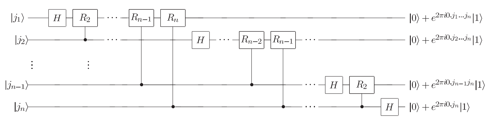
where

\[R_k = \begin{bmatrix}1 & 0 \\ 0 & e^{i2\pi/2^k}\end{bmatrix}\]