An Introduction to de Sitter Space - Part 3

Most of my work is focused on de Sitter space so I want to spend some time focussing on it. Let’s start by describing de Sitter space by picturing it being embedded in a higher dimension space.

We can describe \(dS_d\) (d dimension de Sitter space) by starting with \(\mathbb{R}^{1,d}\) (that is flat space in 1 dimension higher) and then selecting all the points satisfying

\begin{equation} X^\mu X_\mu =-X_0^2 + X_1^2 + …. X_d^2 = l^2 \end{equation}

where l is some number called the de Sitter radius.

To understand this a bit better let’s focus on \(dS_2\) inside \(\mathbb{R}^{1,2}\). We can draw \(\mathbb{R}^{1,2}\) as our standard 3D axis.

Then we can think of de Sitter space as the points \((X_0, X_1, X_2)\) obeying the equation:

\begin{equation} -X_0^2 + X_1^2 + X_2^2 = l^2 \end{equation}

So we find \(dS^2\) is the following hyperboloid:

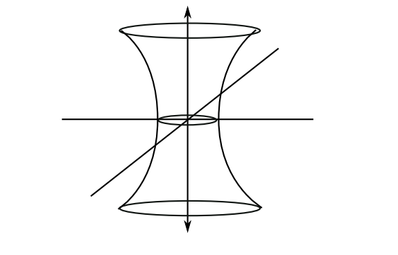
From this picture we can see that there is a circle of a given radius at every value of t (the vertical axis). This generalises to higher dimensions - for every time there is a \(d-1\) sphere and its radius is determined by the time.

We can find some nice co-ordinates for \(dS_n\):

\begin{equation} \tau \in (-\infty, \infty) \end{equation} \begin{equation} \theta_i \in [0, \pi], 1 \leq i < d- 1 \end{equation} \begin{equation} \theta_{d-1} \in [0, 2\pi) \end{equation}

Then these are related to the standard co-ordinates \(X_i\) on \(\mathbb{R}^{1,d}\) in the following way:

\begin{gather} X_0 = \sinh(\tau) \
X_i = \omega_i \cosh(\tau) \end{gather}

where

\begin{equation} \omega_1 = \cos(\theta_1) \end{equation} \begin{equation} \omega_i = (\Pi_{n=1}^{i-1}\sin(\theta_n))\cos(\theta_i) \end{equation}

Now this embedding takes the standard metric on flat space \(\eta = diag(-1,1,1,..1)\) and induces the following metric:

\begin{equation} ds^2 = -d\tau^2 + \cosh (2\tau )d\Omega^2_{d-1} \end{equation}

where \(d\Omega^2_{d-1}\) is the standard metric on the sphere

Causality and Penrose Diagrams

We want to understand the causality of de Sitter space. That is, given signals can’t travel faster than the speed of light who can send signals to who.

To do, this we will draw what is called a Penrose diagram. This involves picking some new co-ordinates for de Sitter which will allow us to draw it on a page.

Since our space is infinite, we need some way of making it finite. And we would like to do this in such a way that light rays (null geodesics) still travel at 45 degrees. This way we can easily figure out which points can send signals to each other by looking at how we can draw 45 degree lines.

To do this we define

\begin{equation} cos(T) = \frac{1}{\cosh(\tau)} \end{equation}

So \(T \in (-\pi/2, \pi/2)\)

Then the metric becomes

\begin{equation} ds^2 = \frac{1}{\cos^2(T)}(-dT^2 + d\Omega^2_{d-1}) \end{equation}

Now we define a new metric

\begin{equation} d\tilde{s}^2 = \cos^2(T) ds^2 = (-dT^2 + d\Omega^2_{d-1}) \end{equation}

This is metric is different to original metric but it is conformally related to it (we say metrics \(da^2, db^2\) are conformally related if \(da^2 = \Omega^2(x)db^2\) for some function \(\Omega\)). The important thing is that null geodesics are the same if two metrics are conformally related. So for our purposes of understanding causality we can just study this new metric.

We can use the fact that \(d\Omega^2_{d-1} = d\theta + \sin^2(\theta)d\Omega^2_{d-2}\) (where \(\theta \in [0, \pi/2]\) to write

\begin{equation} d\tilde{s}^2 = -dT^2 + d\theta + \sin^2(\theta)d\Omega^2_{d-2} \end{equation}

Now let’s just focus on the T and \(\theta\) directions. Plotting these gives use a square with time running upwards.

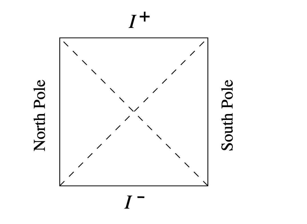
The \(I^-\) and \(I^+\) represent the points at infinite time. The left and right edges represent someone at the north/south pole of the \(S^{d-2}\) sphere at particular time.

Then each point inside the square represents a \(S^{d-2}\) sphere.

Now let’s try to understand what this diagram is telling us.

Someone standing at the north pole, can only send signals to someone they can reach by a line that is at 45 degrees for less to the vertical. So they can’t send a signal to just anyone but only to half the diagram. In fact, they can never send a signal to someone at the south pole in finite time.

Similarly, if we consider who can send signals to the north pole, once again its only half the diagram. And it is different to the half that can receive signals from the north pole. The intersection of these two sections in the wedge on the left hand side and is called the northern causal diamond.

Cosmology

Cosmology is the study of the large scale structure of the universe. It starts from the observation that the universe (or the spatial part of the universe) is homogenous and isotropic (on large scales)

So we expect the spatial part of the metric to be a homogenous, isotropic 3D space.

The other key observation needed for cosmology is that the universe is expanding. This suggests the spatial part of our metric should be scaled by time.

This suggests the metric we should study in Cosmology should be of the form

\begin{equation} ds^2 = -dt^2 + a(t)^2 dl^2 \end{equation}

where \(dl^2\) is the metric on some homogenous, isotropic 3D space.

A homogenous, isotropic 3D space must have constant curvature and this gives us 3 possible choices: positively curved (\(R > 0\)), negatively curved (\(R < 0\)) or flat \((R=0)\).

The positively 3D space has the metric of a sphere so putting that in we get

\begin{equation} ds^2 = -dt^2 + a(t)^2 d\Omega_{3} \end{equation}

This is the metric of de Sitter space! So if the universe is positively curved, then it is described by the de Sitter metric.