The Strong CP Problem A Guide

I recently had to give a talk to other PhD students in the Maths department and I choose to do it on my master’s dissertation. This was on a topic called the Strong CP problem which is a fine tuning problem on particle physics and these are my notes from that talk.

Conventions

We will let greek indices \(\mu, \nu\) etc run over \(0,1,2,3\) where as latin indices will run over \(1,2,3\)

We will also Einstein summation convention, that is repeated indices are summed over. And I will be using the metric \(\eta = diag(-1,1,1,1)\)

What this means is that

\[\sum_{i=0}^3 a_i \eta_{ij}b_j = -a_0b_0 + a_1b_1 + a_2b_2 + a_3b_3 = a_\mu b^{\mu}\]

Principle 1: Natural is lazy

What I mean by this is that nature is lazy.

Imagine I have particle which starts at some position at time t1 and ends at a different position t2 then nature will pick the path \(q(t)\) connecting the two points which minimises a quantity called the action, denoted S

For particles we can really easily write down what S is

\[S[q(t)] = \int_{t_1}^{t_2} dt \frac{1}{2}m\dot{q}^2 - V(q)\]

where the first term is the kinetic energy of the particle and the second term is the potential energy e.g. the energy due to things like gravity. We will call everything inside the integral the Lagrangian and denote it \(\mathcal{L}\).

So nature will always pick the path that minimises this quantity S.

Now this generalises to what are called fields. So instead of having a path

\[q : \mathbb{R} \to \mathbb{R}\]

which eats a time and gives us back a position we can have a function

\[\phi : \mathbb{R}^n \to \mathbb{R}\]

which eats a position in space and time and then gives us back a number.

We can then write an action for a field in a similar way

\[S[\phi] = \int d^nx \partial_\mu \phi \partial^\mu \phi - V(\phi)\]

where this time we’re integrating over space and time.

So in summary, we expect Nature to be trying to minimise something called the action and the action can usually be written of the integral of something called the Lagrangian.

Principle 2: Special Relativity

Special Relativity tells us two things:

1. The laws of physics are the same for all inertial observers
2. The speed of light is constant (in all inertial reference frames)

We can interpret this mathematically, by saying that all fields transform in some representation of \(SO(1,3)\). This means that if we want to describe you looking at a field and me looking at a field, then there should be a representation relating them.

We also want S to be invariant under the combined action of these representations. So if we transform each field in their respective representation then the action S should be unchanged.

We will actually often require \(\mathcal{L}\) to be unchanged which is slightly stronger.

This constraints what we can write in our Lagrangian, we can only have terms that are unchanged under the action of these representations

Principle 3: Gauge invariance

Gauge invariance is the hardest I think of the principles we’ll need to understand it. What is says at its core is that you will have degrees of freedom in your theory which can be changed in some way without affecting the physics.

A Mechanical Example

So to try and understand this, let’s look at an example. Let us imagine we have 4 masses in a plane attached with rigid rods in the following way:

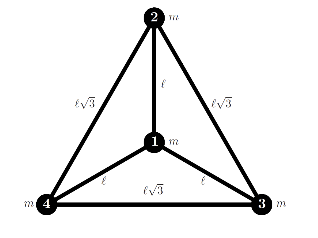
We can write down a Lagrangian for this theory:

\[\mathcal{L} = \frac{m}{2}\sum_{i=1}^4\dot{q}_i - \frac{1}{2} \sum_{\{i,j\} \in E} q_{\{i,j\}}(||q_i-q_j||^2 - l_{\{i,j\}}^2)\]

where E is the set of edges/rods \(\{ \{1,2\}, \{1,3\}, \{1,4\},\{2,3\},\{2,4\},\{3,4\} \}\)

The first term is just the kinetic energy of the masses. The second term looks strange but it is there to enforce the constraints of the rods being a fixed length. To do this we did introduce this new degree of freedom \(q_{\{i,j\}}\)

Now we can solve the equations of motion for this and we find that

\[q_1(t) = (0,0)\] \[q_2(t) = (-l\sin(\omega t), l\cos(\omega t)) \\\] \[q_3(t) = (-l\sin(\omega t - \frac{2\pi}{3}), l\cos(\omega t)-\frac{2\pi}{3}) \\\] \[q_4(t) = (-l\sin(\omega t+\frac{2\pi}{3}), l\cos(\omega t+\frac{2\pi}{3}))\]

and that

\[q_{\{1,2\}}(t)=q_{\{1,3\}}(t) = q_{\{1,4\}}(t) = f(t)\] \[q_{\{2,3\}}(t)=q_{\{2,4\}}(t) = q_{\{3,4\}}(t) = \frac{1}{3}(m\omega^2 -f(t) )\]

Now f(t) is an arbitrary function of t. Notice that f(t) does not appear in our description of the position of the particles so f(t) does not completely change them. But we have this arbitrary function f(t) which we can alter without changing the physics of our system.

When we have a situation like this, we say we have a gauge redundancy, because we have more one than choice that can lead to the same physics. The important thing is that our Lagrangian stays the same no matter which choice we make (we say our Lagrangian is gauge invariant).

Electromagnetism

Let’s look at another example: electromagnetism. Now the Lagrangian for electromagnetism can be written as

\[\mathcal{L} = \frac{1}{2}(E^2 - B^2)\]

where E is the electric field and B is the magnetic field. Now from this you can get Maxwell’s equations.

But there is another way to write this. Let us introduce the fields:

\[A_\mu : \mathbb{R}^{1,3} \to \mathbb{R}\]

We will define them as obeying

\[E = -\nabla A_0 + \partial_t \hat{A}\] \[B = \nabla \times \hat{A}\]

where \(\hat{A} = (A_1, A_2, A_3)\)

And for convenience, we will define

\[F_{\mu\nu} = \partial_\mu A_\nu - \partial_\nu A_\mu\]

Then we can write the Lagrangian as

\[\mathcal{L} = \frac{1}{4} F_{\mu\nu}F^{\mu\nu}\]

Now this will give us the same equation of motion and therefore the same physics for E and B.

But there is the following redundancy

\[A_\mu(x) \to A_\mu(x) + \partial_\mu \alpha(x)\]

So once again we have the same thing, we have this Lagrangian which leads to the correct physics but there is some arbitrariness. We can choose different \(A_\mu\) and get the same physics out.

Local Symmetry

We can try and ask why we are interested in these kind of gauge theories? Well they arise when we try to consider local symmetries.

What I mean by this, is if we consider a complex scalar field

\[\phi : \mathbb{R}^{1,3} \to \mathbb{C}\]

Then we can write down the following Lagrangian

\[\mathcal{L} = \partial_\mu \phi^*\partial^\mu \phi - \phi^*\phi\]

This has a global U(1) symmetry. That is we do

\[\phi \to e^{i\alpha} \phi\]

Then our Lagrangian is unchanged.

Now we can ask what happens if we promote \(\alpha\) from being a number to being a function of spacetime. So we do

\[\phi \to e^{i\alpha(x)} \phi\]

The potential term will be fine but the derivatives in the kinetic term will be the problem as it will pull down factors of \(\alpha'\)

So people thought about this and what they found is that if you introduce new fields:

\[A_\mu : \mathbb{R}^{1,3} \to \mathbb{R}\]

and define the covariant derivative

\[D_\mu = \partial_\mu - iA_\mu\]

Then you can write down the new Lagrangian

\[\mathcal{L} = D_\mu \phi^* D^\mu \phi\]

which is invariant under the following combination of transformations:

\[\phi \to e^{i\alpha(x)}\phi\] \[A_\mu \to A_\mu + \partial_\mu \alpha(x)\]

So we end up with a theory that has a U(1) local symmetry but to do this we had to introduce these new fields called gauge fields and they had to transform in some special way.

Now the dynamics of the system is unchanged under

\[\phi \to e^{i\alpha(x)}\phi\] \[A_\mu \to A_\mu + \partial_\mu \alpha(x)\]

so we have some kind of gauge redundancy.

Now this process of starting with some global symmetry and turning it into a local symmetry is called gauging a symmetry.

Non Abelian Groups

This process generalises fairly easily to groups other than U(1). But it is slightly more complicated as other Lie groups are non Abelian.

So let’s focus on the case of SU(N). To create a theory with an SU(N) local symmetry we introduce some new fields

\[A_\mu : \mathbb{R}^{1,3} \to \mathfrak{su}(n)\]

This time valued in the Lie algebra of SU(N)

These will expect these to transform as

\[A_\mu \to \alpha(x)A_\mu \alpha^{-1}(x) - i (\partial_\mu \alpha(x))\alpha^{-1}(x)\]

where \(\alpha(x) \in \mathfrak{su}(n)\)

Then we define the covariant derivative as before

\[D_\mu = \partial_\mu - iA_\mu\]

and we can define \(F_{\mu\nu}\) as

\[F_{\mu\nu} = i[D_\mu, D_\nu]\]

Finally, when in our action we have to replace \(F_{\mu\nu}F^{\mu\nu}\) by \(Tr(F_{\mu\nu}F^{\mu\nu})\)

So as an example imagine we have the fields

\[\phi : \mathbb{R}^{1,3} \to \mathbb{C}^3\]

The we could have written down the Lagrangian

\[\mathcal{L} = \partial_\mu \phi^\dagger \partial^\mu \phi\]

Then to promote it to an SU(3) gauge theory we instead write

\[\mathcal{L} = D_\mu \phi^\dagger D ^\mu \phi\]

and we could add

\[\mathcal{L} = D_\mu \phi^\dagger D ^\mu \phi + Tr(F_{\mu\nu}F^{\mu\nu})\]

For most of the rest of the talk we will focus on pure SU(3) gauge theory. So just the \(A_\mu\) fields.

Now for a summary of this section, is that nature likes to be described by theories with gauge redundancy (that is extra degrees of freedom that don’t change the physics e.g. the action) and we can make these theories by trying to turn a global symmetry into a local one.

Principle 4: Whatever can happen will happen

Principle 4 is the idea that anything than can happen will happen and the probability of it happening to related to the following object

\[Z = \int D\phi e^{iS[\phi]}\]

This object is called the path integral and what it does is integrate over all possible field configurations and weights them by \(e^{iS[\phi]}\)

From this object is is possible to find all the probabilities of various things happening.

Putting it all together - SU(3) Gauge Theory

Putting everything we’ve learnt so far together. We want to study pure SU(3) gauge theory (physically, this corresponds to the force in Nature called the Strong force or QCD)

That is we want to write down an action that includes all the combinations of our fields

\[A_\mu : \mathbb{R}^{1,3} \to \mathfrak{su}(3)\]

That are Lorentz invariant and gauge invariant e.g. unchanged under

\[A_\mu \to \alpha(x)A_\mu \alpha^{-1}(x) - i (\partial_\mu \alpha(x))\alpha^{-1}(x)\]

where \(\alpha(x) \in \mathfrak{su}(3)\)

One term we have is

\[Tr(F_{\mu\nu}F^{\mu\nu})\]

which we have been working with all along. But in the spirit of whatever happens, happens we can ask if there are any others?

It turns out there is one more we can consider

\[Tr(\epsilon_{\mu\nu\rho\sigma}F_{\sigma\rho}F_{\mu\nu})\]

This is often called the \(\theta\) term

So we want to study

\[S = \int d^4x Tr(F_{\mu\nu}F^{\mu\nu}) + \theta Tr(\epsilon_{\mu\nu\rho\sigma}F_{\sigma\rho}F_{\mu\nu})\]

Or more accurately we want to understand the path integral where this is the action

\[Z = \int DA_\mu e^{iS[A_\mu]}\]

The Effect of the Theta Term

Now, what is the effect of us including this extra term. Well it has one rather striking consequence - it violates parity.

Parity is the idea that if we flipped all of space in a mirror then does physics remain the same?

If it doesn’t we say parity has been violated. Now our standard term

\[Tr(F_{\mu\nu}F^{\mu\nu})\]

does not violate parity but

\[Tr(\epsilon_{\mu\nu\rho\sigma}F_{\sigma\rho}F_{\mu\nu})\]

does.

So we should be able to look for evidence of this term by going out and looking for parity violation. Now people have done this and they have found there is no parity violation (related to SU(3)) in nature, which means \(\theta\) must be 0.

This is very odd, we expect everything than can happen to happen so having some term ruled out by it just having an zero in front of it is ugly.

Removing the Theta Term

We would like some reason why the theta term is ruled out or has to set to 0.

One way is propose that parity is a symmetry of nature and we can’t have anything that violates it. This was believed for a long time but it was discovered that the weak force (another gauge theory based on SU(2)) violates parity.

Another way, that you might have thought of is to notice that the theta term is actually total derivative as it can be written as

\[\int d^4x \partial_\mu \epsilon^{\mu\nu\rho\sigma} Tr(A_\nu \partial_\rho A_\sigma + \frac{2}{3}A_\nu A_\rho A_\sigma)\]

This means that we should only get contributions to the action from the values of the field at the boundary of spacetime. So if the contribution at the boundary of spacetime turns out be 0 then this term won’t contribute anything. Sadly, you can construct field configurations (called instantons) where the contribution from this term is non zero.

Axion

So it seems like we’re stuck with this term, but people thought about it and came up with another way to try and get rid of it. And the solution we’re going to look at is called the Axion.

The axion starts the following assumptions:

There is a scalar field

\[a : \mathbb{R}^{1,3} \to \mathbb{R}\]

which has two nice properties.

Firstly, at low energies this field is approximately 0 (the fancy term is that is has a 0 Vacuum Expectation Value). Secondly, it has a strange symmetry

\[a \to a + \frac{\kappa}{f_a}\]

where \(\kappa\) and \(f_a\) are just some numbers. This means we can shift the field by some constant and nothing changes.

Now, if we have a field with these properties then we can do the following.

We can couple it our \(\theta\) term so we have

\[a(x)Tr(\epsilon_{\mu\nu\rho\sigma}F_{\sigma\rho}F_{\mu\nu}) + \theta Tr(\epsilon_{\mu\nu\rho\sigma}F_{\sigma\rho}F_{\mu\nu})\]

Then using our shift symmetry we can remove the theta term so we are left with

\[a(x)Tr(\epsilon_{\mu\nu\rho\sigma}F_{\sigma\rho}F_{\mu\nu})\]

which at low energies is 0 as at low energies a is 0.

Now this solution seems very odd. Instead of just accepting that some number is 0, we have posited that there exists some extra field with some strange symmetry properties.

Worse than this, the axion theory as we have written it now is not renormalizable, what this means is that you end up with a bunch of nasty infinities if you try and calculate with this theory at arbitrarily high energies.

So what we would like is some theory, that in the low energy limit (what physicists call the IR) reduces to this axion theory.

KSVZ Axion

It turns out this has been found (in fact many have) and the simplest one is called the KSVZ axion.

The key idea of it to introduce a complex scalar field with a U(1) global symmetry then use two ideas which we won’t have time to cover: Chiral Anomaly and Spontaneous Symmetry Breaking. To get the correct low energy behaviour.

Why do people like it?

The axion solution is popular for a few reasons. Firstly, it solves this Strong-CP problem. Secondly, it is a candidate for dark matter. Finally, the appear in String Theory models.